Linear models for classifications

4.1.3 Least squares for classification

Matrices legend.

Matrix	Dimension
$\tilde{W}$	$(D+1)\times K$
$\tilde{X}$	$N\times (D+1)$
$T$	$N\times K$

Consider a classification task with $K$ classes, let $t$ be a one-hot encoding target vector. Each class $C_k$ is described by its own linear model so that

$$y_k(x)=w_k^{T}x+w_{k_0}k=1,\dots ,K$$

By using vector notation, we can combine them together:

$$y(x)=W^{T}x$$

Where $W$ is a $(D+1)\times K$ matrix such that the $k$-th column is $(w_{k_0},w_k^T{)}^T$ and $x=(1,x^T{)}^T$.

Objective: to determine the parameters of $\tilde{W}$ by minimizing a sum-of-squares loss function.

Consider a training dataset $\{x_n,t_n{\}}_{n=1}^N$ and define two sparse matrices

• $T$ of dimension $N\times K$ such that the $n$-th row is the binary one-hot-encoded vector $t_k$.
• $X$ of dimension $N\times (D+1)$ such that the $n$-th row is $x_n^T$

The sum-of-squares loss function can be written as:

$$E_D(W)=\frac{1}{2}\text{Tr}\left\{(XW-T{)}^T(X\tilde{W}-T)\right\}$$

Question: why do we use the trace?

Set the derivative of $E_D$ w.r.t. $\tilde{W}$ to zero and obtain the following solution:

$$W=(X^{T}X{)}^{-1}{X}^{T}T=({\tilde{X}}^{†}{)}^{T}T$$

If we want to obtain the result without using too much matrix calculus we can do the following:

$$\begin{array}{rl}XW& =T\\ X^{T}XW& =X^{T}T\\ (X^{T}X{)}^{-1}{X}^{T}XW& =(X^{T}X{)}^{-1}{X}^{T}T\\ W& =(X^{T}X{)}^{-1}{X}^{T}T\\ W& =X^{†}T\end{array}$$

The discriminant function will be:

$$y(x)=W^{T}x=T^T(X^{†}{)}^{T}x$$

Problems with the discriminant function obtained through minimization of SSE:

• Sensible to outliers
• Bad performances since it estimates $\mathbb{E}[t\mid x]$ under assumption of Gaussian noise, which is clearly wrong when estimating a binary vector $t_n$

An interesting property

Every target vector in the training set satisfies some linear constraint:

$$a^T{t}_n+b=0$$

For some costants $\bar{a},b$. The model prediction for any value of $x$ will satisfy the same constraint

$$a^{T}y(x)+b=0$$

If we use a one-hot-encoding scheme for $t_n$, then components of $y(x)$ will sum up to 1. However, this is not enough for considering $y(x)$ a probability distribution since its components are no bound to $[0,1]$.

4.1.4 Fisher's linear discriminant

Suppose we have 2 classes, the idea is to project the D-dimensional input $x$ to a scalar value $y=w^{T}x$ and classify $x$ as class $C_1$ if $y\ge -w_0$ and class $C_2$ otherwise.

The problem is that projecting the input from D dimensions to 1 dimension consists on a significant loss of information, and if the classes are well separated in the high-dimensional space, they can overlap in the 1-dimensional space. However, we can optimize $w$ in order to maximize the separation between classes in the 1-dimensional space.

One way to do this is to consider the class mean vectors:

$${\bar{m}}_1=\frac{1}{N_1}\sum _{n\in C_1}{x}_n{\bar{m}}_2=\frac{1}{N_2}\sum _{n\in C_2}{x}_n$$

And maximize

$${\hat{m}}_2-{\hat{m}}_1=w^T({\bar{m}}_1-{\bar{m}}_2)$$

where ${\hat{m}}_k=w^T{\bar{m}}_k$. One problem is that we can make ${\hat{m}}_k$ arbitrarly large by incrementing the magnitude of $w$. This can be solved by constraining a fixed magnitude ${\sum }_i{w}_i^2=1$. To enforce this constraint during optimization, we can use Lagrange multipliers. We find that $w\propto ({\bar{m}}_2-{\bar{m}}_1)$.

The problem with this simple approach is that it doesn't take the variance into account, and the datapoints in the 1-dimensional space may be overlapped (e.g., when their distribution has a strongly nondiagonal covariance). See the figure on the left below.

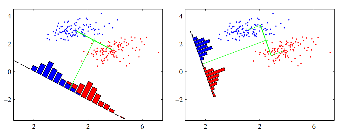
The discriminant function on the right is obtained using the Fisher linear discriminant, which introduce the variance in the objective to optimize.

Define the variance of class $k$ in the projected space as:

$$s_k^2=\sum _{n\in C_k}(y_n-{\hat{m}}_k{)}^2$$

where $y_n=w^T{x}_n$. The total within-class variance for the whole dataset is simply $s_1^2+s_2^2$. The fisher criterion to maximize is defined as the ratio of the between-class variance to the within-class variance:

$$J(w)=\frac{({\hat{m}}_2-{\hat{m}}_1{)}^2}{s_1^2+s_2^2}$$

We can rewrite the Fisher criterion in the following form to make the dependence on $w$ explicit:

$$J(w)=\frac{w^T{S}_{B}w}{w^T{S}_{W}w}$$

Where $S_B$ is the between-class covariance matrix:

$$S_B=({\bar{m}}_2-{\bar{m}}_1)({\bar{m}}_2-{\bar{m}}_1{)}^T$$

and $S_W$ is the total within-class covariance matrix:

$$S_W=\sum _{n\in C_1}(x_n-{\bar{m}}_1)(x_n-{\bar{m}}_1{)}^T+\sum _{n\in C_2}(x_n-{\bar{m}}_2)(x_n-{\bar{m}}_2{)}^T$$

By differentiation, we find that $J(w)$ is maximized when

$$(w^T{S}_{B}w)S_{W}w=(w^T{S}_{W}w)S_{B}w$$

Since we only care about the direction of $w$, we can drop the scalar factors $(w^T{S}_{B}w)$ and $(w^T{S}_{W}w)$. Then we multiply both sides by $S_W^{-1}$ and obtain the Fisher Linear Discriminant:

$$w\propto S_W^{-1}({\bar{m}}_2-{\bar{m}}_1)$$

If the within-class variance is isotropic, so that $S_W$ is proportional to the unit matrix, then we find that $w$ is proportional to the difference of the class means.

The projection function $y(x)=w^{T}x$ is not really a discriminant, but we can construct a discriminant by choosing a threshold $y_0$ to classify the points.

Relation to least squares

For the two class problem, the Fisher criterion can be obtained as a special case of least squares.

Let $N$ be the total number of observations, $N_1$ the observations from $C_1$ class, and $N_2$ from $C_2$ class. Reparameterize the target values as:

1. $t_n=N/N_1$ if $x_n\in C_1$
2. $t_n=-N/N_2$ if $x_n\in C_2$

Write the sum of squares error function:

$$E=\frac{1}{2}\sum _{n=1}^N[(w^T{x}_n+w_0)-t_n{]}^2$$

By setting $\partial E/\partial w_0=0$ and $\partial E/\partial w=0$, after some algebraic manipulations, we find:

$$w\propto S_W^{-1}(m_2-m_1)w_0=-w^{T}m$$

where $w$ corresponds to the solution for the Fisher criteria, and we have also obtained an expression for the threshold $w_0$, where $m$ is the mean of all the observation. For intermediate steps, check page 210.

Fisher discriminant for multiple classes

Suppose $K>2$ classes. Let $x_n\in {\mathbb{R}}^D$, where $D>K$. We need to project the observation $x_n$ to $y_n\in {\mathbb{R}}^{D^{\prime }}$, and we can calculate each component $y_n^{(k)}$ as follows

$$y_n^{(k)}=w_k^T{x}_n$$

Where $w_k\in R^D$. We can group $w_k$ for $k=1,\dots ,D^{\prime }$ as columns of a matrix $W$ of dimension $D\times D^{\prime }$, and calculate the $y_n$ vector in one step as:

$$y_n=W^T{x}_n$$

Let's define the within and between class covariances for the multi-class problem.

The within class covariance $S_W$ is:

$$S_W=\sum _{k=1}^K{S}_k{S}_k=\sum _{n\in C_k}(x_n-m_k)(x_n-m_k{)}^T{m}_k=\frac{1}{N_k}\sum _{n\in C_k}{x}_n$$

The between class covariance $S_B$ is:

$$S_B=\sum _{k=1}^K{N}_k(m_k-m)(m_k-m{)}^{T}m=\frac{1}{N}\sum _{n=1}^N{x}_n$$

Now let's define the covariances but in the projected space of $y_n$.

The within class covariance $S_W$ is:

$$s_W=\sum _{k=1}^K\sum _{n\in C_k}(y-{\mu }_k)(y-{\mu }_k{)}^T{\mu }_k=\frac{1}{N_k}\sum _{n\in C_k}{y}_n$$

The between class covariance $S_B$ is:

$$s_B=\sum _{k=1}^K{N}_k({\mu }_k-\mu )({\mu }_k-\mu {)}^T\mu =\frac{1}{N}\sum _{n=1}^N{y}_n$$

There exist different objective functions to maximize, but here we use the one from (Fukunaga, 1990), which is:

$$J(W)=\text{Tr}(s_W^{-1}{s}_B)$$

Rewriting with explicit dependence on $W$:

$$J(W)=\text{Tr}\left((W{S}_{W}W{)}^{-1}(W{S}_{B}W)\right)$$

Solution: the columns of the matrix $W$ that maximizes $J(W)$ are the D' eigenvectors of the D' largest eigenvalues of the matrix $S_W^{-1}{S}_B$.

Observation: Since the matrix resulting from an outer product of non-zero vector has always a rank of 1, since $S_B$ is composed by the sum of $K$ rank-1 matrices and since only $K-1$ of these matrices are independent, then $S_B$ as a rank at most equal to $K-1$, and therefore there are at most $K-1$ non-zero eigenvalues. This means that we are unable to find more than $K-1$ linear features by this method (Fukunaga, 1990).

Right now we have only reduced the dimensionality of the data. Where is the discriminant function?

4.1.7 Perceptron

Find my notes about Perceptron here (in italian).

4.2 Probabilistic Generative Models

Consider the binary classification task. We want to compute the posterior probability $p(C_1\mid x)$:

$$\begin{array}{rl}p(C_1\mid x)& =\frac{p(x\mid C_1)p(C_1)}{p(x\mid C_1)p(C_1)+p(x\mid C_2)p(C_2)}\\ & =\frac{1}{\frac{p(x\mid C_1)p(C_1)+p(x\mid C_2)p(C_2)}{p(x\mid C_1)p(C_1)}}\\ & =\frac{1}{1+\frac{p(x\mid C_2)p(C_2)}{p(x\mid C_1)p(C_1)}}\\ & =\frac{1}{1+\exp \left[\ln \frac{p(x\mid C_2)p(C_2)}{p(x\mid C_1)p(C_1)}\right]}\\ & =\frac{1}{1+\exp \left[-\ln \frac{p(x\mid C_1)p(C_1)}{p(x\mid C_2)p(C_2)}\right]}\\ & =\frac{1}{1+\exp (-a)}=\sigma (a)\end{array}$$

Where $\sigma (a)$ is the sigmoid function, which has the property $\sigma (-a)=1-\sigma (a)$.

The inverse of the logistic sigmoid is given by the logit function:

$$a=\ln \left(\frac{\sigma }{1-\sigma }\right)$$

It represents the log of the ratio of probabilities $\ln [p(C_1\mid x)/p(C_2\mid x)]$ for the two classes.

For $K>2$ classes, we have:

$$p(C_k\mid x)=\frac{p(x\mid C_k)p(C_k)}{{\sum }_{j}p(x\mid C_j)p(C_j)}=\frac{\exp (a_k)}{{\sum }_{j}exp(a_j)}$$

where the quantities $a_k$ are defined as:

$$a_k=\ln p(x\mid C_k)p(C_k)$$

This function, called normalized exponential, is also known as the softmax function.

Continuous inputs

Assume that

• $x$ is continuous
• Class conditional densities are Gaussian
• They share the same covariance matrix $\Sigma$

$$p(x\mid C_k)=\mathcal{N}({\mu }_k,\Sigma )$$

Consider the binary classification task. From the results above, we have:

$$p(C_1\mid x)=\sigma (w^{T}x+w_0)$$

Where:

$$w={\Sigma }^{-1}({\mu }_1-{\mu }_2)w_0=-\frac{1}{2}{\mu }_1^T\Sigma {\mu }_1+\frac{1}{2}{\mu }_2^T\Sigma {\mu }_2+\ln \frac{p(C_1)}{p(C_2)}$$

Hence we have that the argument of the activation function is linear w.r.t. the input $x$.

Since the decision boundaries are defined as the areas where $p(C_k\mid x)$ is constant, and since this depends only on the argument of the sigmoid, which is linear w.r.t. $x$, therefore the decision boundaries are also linear w.r.t. $x$.

Changing the prior probabilities will only shift the decision boundaries, since they appear only in the bias parameter $w_0$.

For $K$ classes, we have

$$a_k(x)=w_k^{T}x+x_{k0}$$

where

$$w_k={\Sigma }^{-1}{\mu }_k{w}_{ko}=-\frac{1}{2}{\mu }_k^T{\Sigma }^{-1}+\ln p(C_k)$$

Relaxing the assumption of a shared covariance matrix and considering a different covariance matrix ${\Sigma }_k$ for each class will result in a quadratic dependency w.r.t. of $P(C_k\mid x)$ w.r.t. $x$ (also called quadratic discriminant).

Maximum likelihood solutions

See the derivations at page 220. Suppose we have $N$ samples $x_1,\dots ,x_N$ and their binary class labels $t_1,\dots ,t_N$, where $t_n\in \{0,1\}$, suppose $N_1$ samples belong to class $C_1$ and $N_2$ to class $C_2$. If we condire Gaussian class conditional densities $p(x\mid C_1)=\mathcal{N}(x\mid {\mu }_1,\Sigma )$ and $p(x\mid C_2)=\mathcal{N}(x\mid {\mu }_2,\Sigma )$ with shared covariance matrix $\Sigma$, then the maximum likelihood likelihood solutions are:

• $p(C_1)=N_1/N$
• $p(C_2)=N_2/N$
• ${\mu }_1$ centroid of samples from class $C_1$
• ${\mu }_2$ centroid of samples from class $C_2$
• $\Sigma$ sum of covariance matrices of $C_1$ and $C_2$ weighted by the priors.

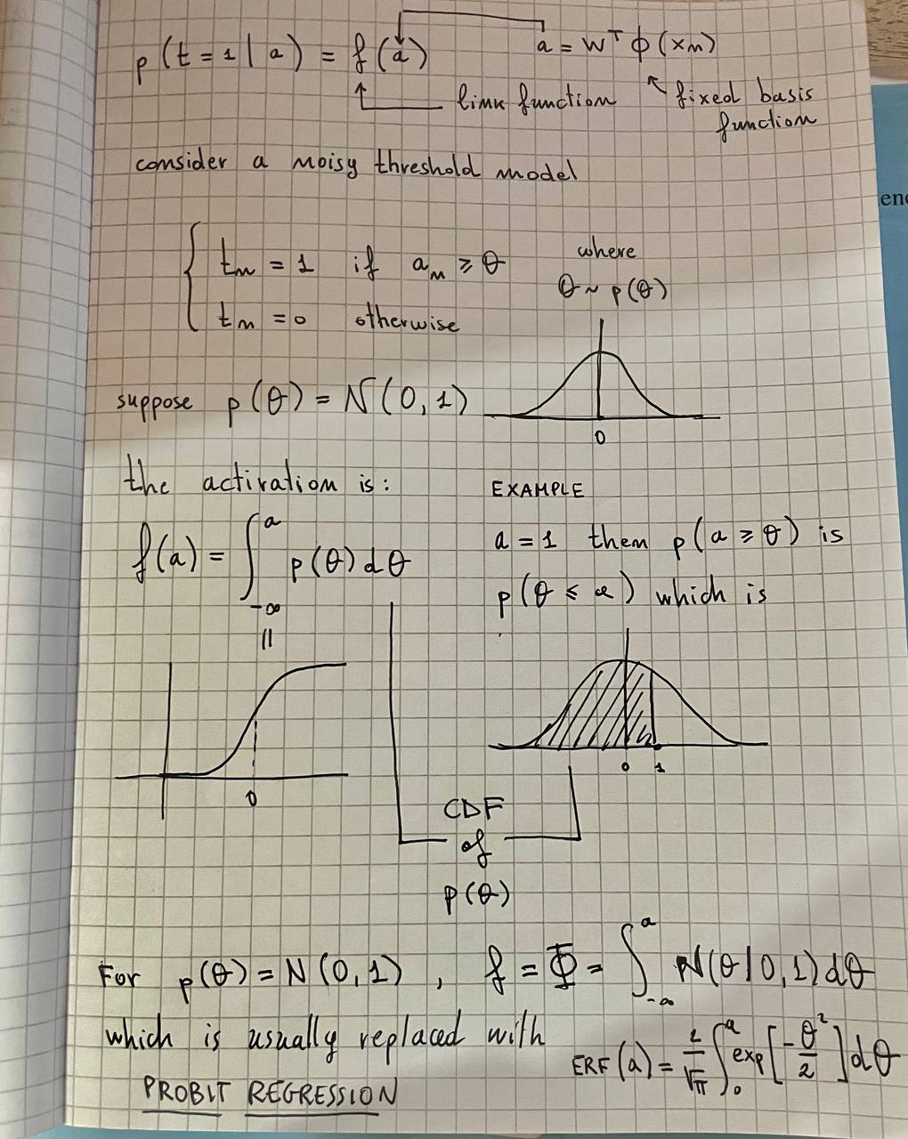
Probabilistic Discriminative Models

Probit regression